Why Past ENSO Cases Aren’t the Key to Predicting the Current Case

Lately, many of us are wondering if a 2014-15 El Niño is going to materialize, and if so, how strong it might become and how long it will last. It might cross some folks’ minds that the answer to these questions can be found by collecting past ENSO cases that are similar and see what happened. Such an approach is known as analog forecasting, and on some level it makes intuitive sense.

In this post, I’ll discuss why the analog approach to forecasting often delivers disappointing results. Basically, it doesn’t work well because there are usually very few, if any, past cases on record that mimic the current situation sufficiently closely. The scarcity of analogs is important because dissimilarities between the past and the present, even if seemingly minor, amplify quickly so that the two cases end up going their separate ways.

Past Cases (Analogs) Similar to 2014

The current situation is interesting because it seems we have been teetering on the brink of El Niño, as our best dynamical and statistical models keep delaying the onset but yet continue to predict the event starting in fairly short order. Which raises the question: have there been other years that have behaved similarly to 2014? Before we check, let’s talk for a minute about how we find good analogs for the current situation.

The set of criteria by which the closest analogs are selected is a contested issue in forecasting.  One can select years based on time series, maps, or among many variables across different periods of time. There are also many different ways to measure similarity, and one has to select the appropriate level of closeness to past cases—in other words, decide how close is close enough.

One main criticism of analog forecasting is the subjectivity of making such choices, which can lead to different answers.  Here, I will use one method based on similarities of sea surface temperature (SST) in the Nino3.4 region (1). Figure 1 shows six other years during the 1950-2013 period that have behaved similarly to this year in terms of SST, and also shows what happened in the seven months following September.

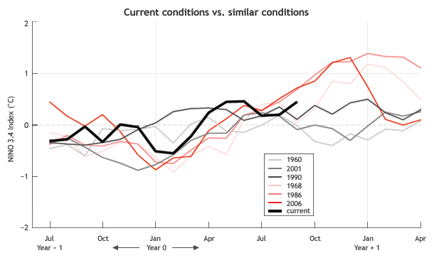
Figure 1. Monthly average SST anomaly in the Nino3.4 region over the last 15 months for this year (thick black line), and the same for 6 other years selected as the closest analogs for this year. After September, the last month for which we have observations for this year, the ENSO behavior of the chosen analog cases is shown for the following seven months, providing a basis for a possible analog forecast for the current year. Photo credit: IRI, Columbia University and NOAA Climate Program Office.

In checking out the analog forecast possibilities in Fig. 1, it is clear that the outcomes are diverse. Out of the six selected cases, three indicate ENSO-neutral for the coming northern winter season, while the other three show El Niño (at least 0.5˚ anomaly)—and all three attain moderate strength (at least 1˚C anomaly) for at least one 3-month period during the late fall or winter (2). For the coming January, the 6 analogs range from -0.3 to 1.4˚C, revealing considerable uncertainty in the forecast (3).

Although this uncertainty in outcomes is somewhat smaller than that what we would have if we selected years completely randomly from the history, it is larger than that from our most advanced dynamical and statistical models. This is one reason analog forecasting systems have been largely abandoned over the last two decades as more modern prediction systems have proven to provide better accuracy.

Why Analogs Often Don’t Work Well

The large spread among the six analog cases selected for a current ENSO forecast is not unusual, and it would be nearly as large even if we came up with a more sophisticated analog ENSO forecast system (4). The big problem in analog forecasting is the lack of close enough analogs in the pool of candidates.

Furthermore, the criteria by which we select cases always ignore some relevant information, and this missed information introduces differences between the current case and the past analog cases. Even if we knew and included everything that did matter, the fact that the ocean and atmosphere are fluids means that tiny differences between the current and past cases often quickly grow into larger differences.

Van den Dool (1994)’s ”Searching for analogs, how long must we wait?” calculates that we would have to wait about 10³⁰ years to find 2 observed atmospheric flow patterns that match to within observational error over the Northern Hemisphere. While the ocean is not as changeable as the atmospheric flow, it is clear that finding close matching analogs would also require a very long historical dataset.

Even finding good matches with the relatively simple Nino3.4 time series is an obstacle (see the left side of Fig. 1).  In the case of ENSO, there are only ~60 years in the “well observed” historical record of tropical Pacific sea surface temperatures and even fewer cases of El Niño or La Niña years. The severe shortness of the past record prevents an analog approach from bearing much fruit. More complex statistical and coupled ocean-atmosphere dynamical models can make better predictions than analogs.

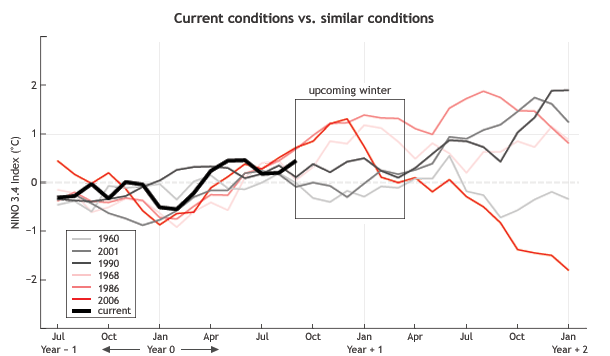
Figure 2. Monthly average SST anomaly in the Nino3.4 region over the last 15 months for this year (thick black line), and the same for 6 other years selected as the closest analogs for this year. This figure goes 9 months farther out into the future than Fig. 1, and most of the future portion of Fig. 1 is contained in the box labeled “upcoming winter”. Note that the medium-bright red line, for 1986-87, shows the rare event of two consecutive years of El Niño, and that the very light red line, for 1968-69, shows a weaker case of the same. Photo credit: IRI, Columbia University and NOAA Climate Program Office.

Yet, despite the above warning, forecasters continue to enjoy identifying analogs when we consider what ENSO might have up its sleeve for the forthcoming seasons. For example, notice in Fig. 2, which shows what happened with each of the 6 analogs nine months farther into the future than shown in Fig. 1, that in early autumn 1986 (medium red line), a late-starting El Niño attained moderate strength during 1986-87, but also continued for a second year and reached even greater strength in 1987-88.

Do late-starting El Niño events tend to endure into a second ENSO cycle and take two years instead of one to run their course? While that is a topic for another post, let’s just say that there have been so few cases of two-year events that it would be foolhardy to actually predict one without more evidence. Interestingly, though, two of the models on this month’s IRI/CPC ENSO forecast plume (Fig. 3) do suggest the possibility of an El Niño both this year and a second year (2015-16). One of those models is NOAA/NCEP’s own CFSv2, and another is the Lamont-Doherty Earth Observatory (LDEO) intermediate model. Could they be on to something?

Figure 3. ENSO prediction plume from September 2014 (see official version of this graphic), for SST anomaly out to Jun-Jul-Aug 2015. The orange lines show predictions of individual dynamical models, and blue lines those of statistical models; the thicker lines show the averages of the predictions from those two model types. The black lines and dots on the left side show recent observations. A weak El Niño (SST of at least 0.5˚, but less than 1˚C anomaly) continues to be predicted for late fall and winter 2014-15 by many of the dynamical and statistical models. The NCEP CFSv2 and the LDEO dynamical models, highlighted in brighter orange, suggest continuation and intensification of El Niño in spring 2015, presaging a possible 2-year event, as occurred in 1986-87-88 (but the LDEO model holds back on a full-fledged El Niño for the first year).

Footnotes

(1) This method uses the 13 months prior to (and including) the most recently completed month, but weights the more recent months more heavily than the less recent ones. In the case of Fig. 1, the relative weights from September 2013 through September 2014 are .02, .02, .03, .05, .06, .06, .07, .09, .10, .11, .12, .14, and .13. This weighting pattern was based on correlations between the earlier and current SSTs, averaged over all starting/ending times of the year. In a more refined system, the weighting pattern would change noticeably depending on these starting/ending times of the year. This variation exists due to the typical seasonal timing of ENSO events. For example, the correlation between SST in February with that in July is low, while the correlation between SST in September with that in February is quite a bit higher, as many ENSO events begin during summer and last through the following winter.

So, as we might expect from the weighting pattern, the similarity between this year and the selected analog years is seen in Fig. 1 to be greatest over the most recent 3 to 5 months. The closeness of the match is calculated as the square root of the sum of the weighted squared differences between the Nino3.4 SST this year and the candidate year. This metric is often called the Euclidean distance, and the smaller the number, the better the analog match.

(2) The time unit used in this analog prediction system is 1-month, in contrast to the 3-month averages usually used by NOAA in ENSO diagnostics and prediction.

(3) This spread is occurring at a time of year when persistence (i.e., maintenance over time of either positive or negative anomalies of SST) is typically strong and so forecasts using just recent observations generally do better than at other times of the year.

(4) More sophisticated analog systems used in earlier decades for seasonal climate forecasting are documented in Barnett and Preisendorfer 1978, Livezey and Barnston 1988, and Barnston and Livezey 1989.

References

Barnett, T. P., R. W. Preisendorfer, 1978: Multifield analog prediction of short-term climate fluctuations using a climate state vector, J. Atmos. Sci., 35, 1771–1787.

Barnston, A. G., and R. E. Livezey, 1989: An Operational Multifield Analog/Anti-Analog Prediction System for United States Seasonal Temperatures. Part II: Spring, Summer, Fall and Intermediate 3-Month Period Experiments. J. Climate, 2, 513–541.

Livezey, R. E., and A. G. Barnston, 1988: An operational multifield analog/antianalog prediction system for United States seasonal temperatures: 1. System design and winter experiments. J. Geophys. Res., Atmospheres, 93, D9, 10953–10974. DOI: 10.1029/JD093iD09p10953

Van den Dool, H. M., 1994: Searching for analogues, how long must we wait?  Tellus A, 46, 314-324.