Butterflies, rounding errors, and the chaos of climate models

First things first—many thanks to our newest ENSO blogger, Nat Johnson, for covering the top-of-the-month post this month while I was scuba diving with manta rays.

Diving in Kona. Photograph by Glen Becker.

This also frees me up to write a post I’ve been thinking about for a while: an entire post about dynamical climate models! Models are a critical tool for climate forecasters, but I haven’t had enough column inches to get into how they really work.

What’s a model? Not this kind…

Used with Creative Commons license. Henry Jose, photographer.

If you say “model” to a weather or climate forecaster, she’ll immediately think of a computer program that takes in information on current conditions and outputs a picture of potential future conditions. Here, I’ll be talking about dynamical models, which use complex physical equations to predict the future, rather than statistical models. Statistical models are simpler, and use historical observations and their relationships to predict how conditions might evolve. Tony has a brief explanation of statistical models in the notes of this post.

A little bit of history

Dynamical models have only become feasible in the last couple of decades because supercomputers are required to crunch through all of the observational input data and mathematical equations they use. The earth system (atmosphere, ocean, land, and ice) changes in a chaotic manner. Here, chaos doesn’t mean “essential randomness,” but rather that very small—seemingly insignificant—differences in the input can result in a large difference in the output.

The origin of modern dynamical models lies in experiments done in the 1950s on some very early computers. Edward Lorenz, one of the pioneers in weather prediction, used some relatively simple equations to predict how current conditions would evolve. He would input some information about the current weather—e.g. temperature, winds, pressure—and the computer would solve the equations, giving a picture of how the weather would change in time.

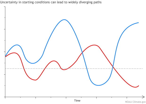
As often happens in science, he made a big discovery by accident. He repeated his first experiment, but rounded off the numbers to three decimal points instead of six. So, for example, instead of telling the computer that the temperature was 27.084271°, he input 27.084°. He expected that this tiny difference would be insignificant, and was surprised to find that, after a short time, the results of the two experiments diverged dramatically.*

Example illustration showing two different paths originating from very close initial points. Illustration by climate.gov.

Lorenz spent many years studying this effect, which has worked its way into popular culture—the “butterfly effect,” named after a talk he gave in 1972. The idea is that tiny changes have unpredictable effects: the flap of a butterfly’s wings in Brazil could set in motion atmospheric events that lead to a tornado forming in Texas several weeks later. Since we can’t possibly know precisely what every butterfly will do, we can’t precisely predict the future.

Fake nature

Climate models simulate this chaotic property of nature with mathematical equations. Processes like the movement of air, evaporation and condensation of water, heat transfer, and the complex interactions between different elements of the system are all described by these equations. The processes that are too small or too complex to be represented by known physical equations are approximated, or “parameterized.” For example, the movement of clouds is parameterized in models. The current observed climate conditions are the starting point for all the equations—the initial conditions—and the end point is a potential scenario for future climate conditions. Chickens go in, pies come out.

In order to get a perfect forecast, we would have to know the exact conditions of every single molecule in the global system and use them as input for a colossal computer model that had an exact mathematical representation of every physical process.

Not only is this impossible in a practical sense, it disobeys a basic principle of physics, the Heisenberg uncertainty principle, which states that we can never know both the exact location and velocity of tiny particles, essentially because in trying to measure them, we’ll change them.

But they’re still useful!

Since we can’t know what every single butterfly is doing or is going to do, let alone the temperature of every atom in the Pacific ocean, what’s the use? Well, in climate prediction, we aren’t trying to forecast specific weather conditions, but rather the average over some period of time—a month, season, year, or longer.

To do this, we run the model many times, each time giving it a slightly different set of initial conditions, resulting in an ensemble of outcomes. The slightly different inputs represent our inexact knowledge of the current conditions. The outcomes will all be different—and they’ll be a lot further apart than the sets of initial conditions were, because of the chaos in the system. However, in most cases the forecasts will show a common theme: the signal that emerges from the noise.

For example, say we would like to forecast the development of the sea surface temperature in the central Pacific. We run the model, telling it the current temperature, winds, subsurface temperatures, and how they’ve changed recently. Then we’ll run it again, after changing the input slightly. Rinse and repeat!

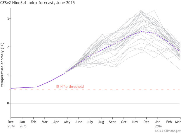
CFSv2 forecast for Nino3.4 sea surface temperature anomaly (departure from long-term mean), made in June 2015. Gray lines show 32 individual model runs, and purple dashed line shows average of all.  Solid purple line is the observed sea surface temperature anomaly.

In this example, the model runs trend upward, toward a strengthening El Niño. Some ensemble runs predict more warming, others less, but the overall signal is in the direction of warming. I’m running out of space here, but for more info on ensemble models and signal versus noise, check out Michelle’s great post, and Tony’s about why our forecasts are probabilistic.

A forecast forecast

There are still a lot of improvements to be made in climate models, such as more accurate physical equations. (For example, improving the representation of clouds.) In fact, the inaccuracies in the equations are also a cause of forecast divergence. But that is a topic for another post! Also, while we will never know the exact state of every element of the initial conditions, improved coverage of observations (TAO shout-out) will help refine, and hopefully improve, the model output.

Today’s models are much more advanced than the previous generation, and model development is a very active research area. Hopefully we can look forward to seeing more sophisticated models strut their stuff on the future catwalk.

* For more on Ed Lorenz’s life and work, check out the in memoriam article written by T. N. Palmer and published in Biographical Memoirs of the Royal Society.