Exactly the same, but completely different: why we have so many different ways of looking at sea surface temperature
As Emily has painstakingly documented at the beginning of every month for what seems like an eternity, we have an El Niño event on our hands. And if you’ve read her posts religiously (which of course you have, because they are awesome), you already know that one way Emily shows the strength of El Niño is via the sea surface temperature (SST) anomalies in a region of the Pacific Ocean called the Niño3.4 region.
You may also have noticed that when we talk about how one event compares to another, we usually say something like, “Depending on what dataset you use….” Up until now, though we’ve haven’t talked much about how exactly we determine which sea surface temperature dataset to use to determine El Niño’s strength.
If your first reaction to that last sentence was “Wait, there are different sea surface temperature datasets?” you are not alone. But yes, it’s true. At the Climate Prediction Center (CPC) alone, we routinely refer to at least a couple of different datasets. And scientists around the world have others.
It would seem logical to compare these SST values to each other in the present and to those during past events. They refer to the exact same thing, at the exact same time, in the exact same region of the Pacific Ocean. They must be interchangeable, right? They’re not. Heck, for some datasets, it’s not even advisable to compare Niño3.4 anomalies for one year to previous years within the same dataset! Whhaaattt?
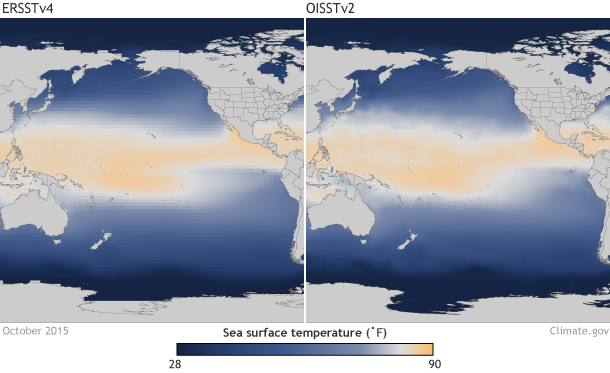
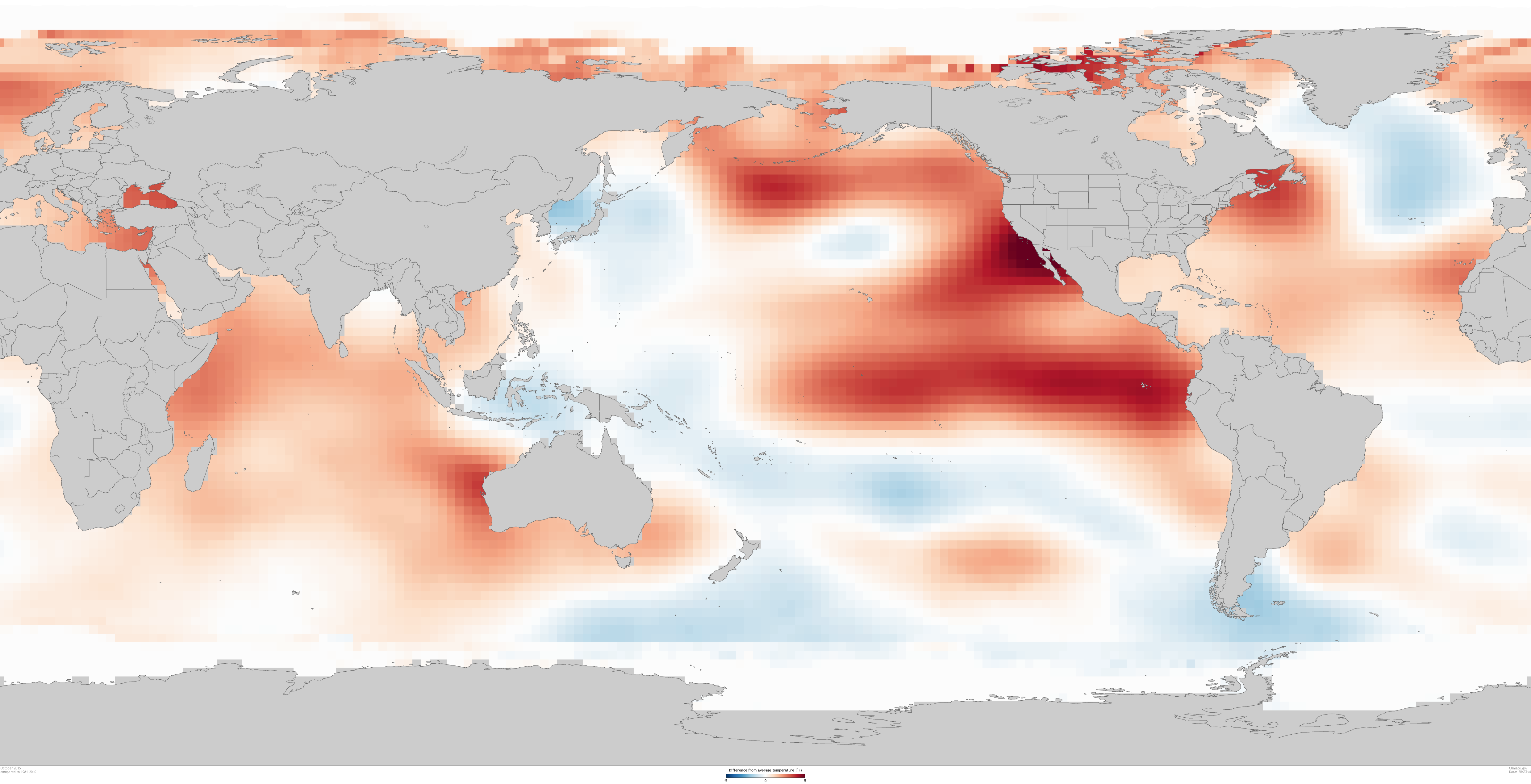
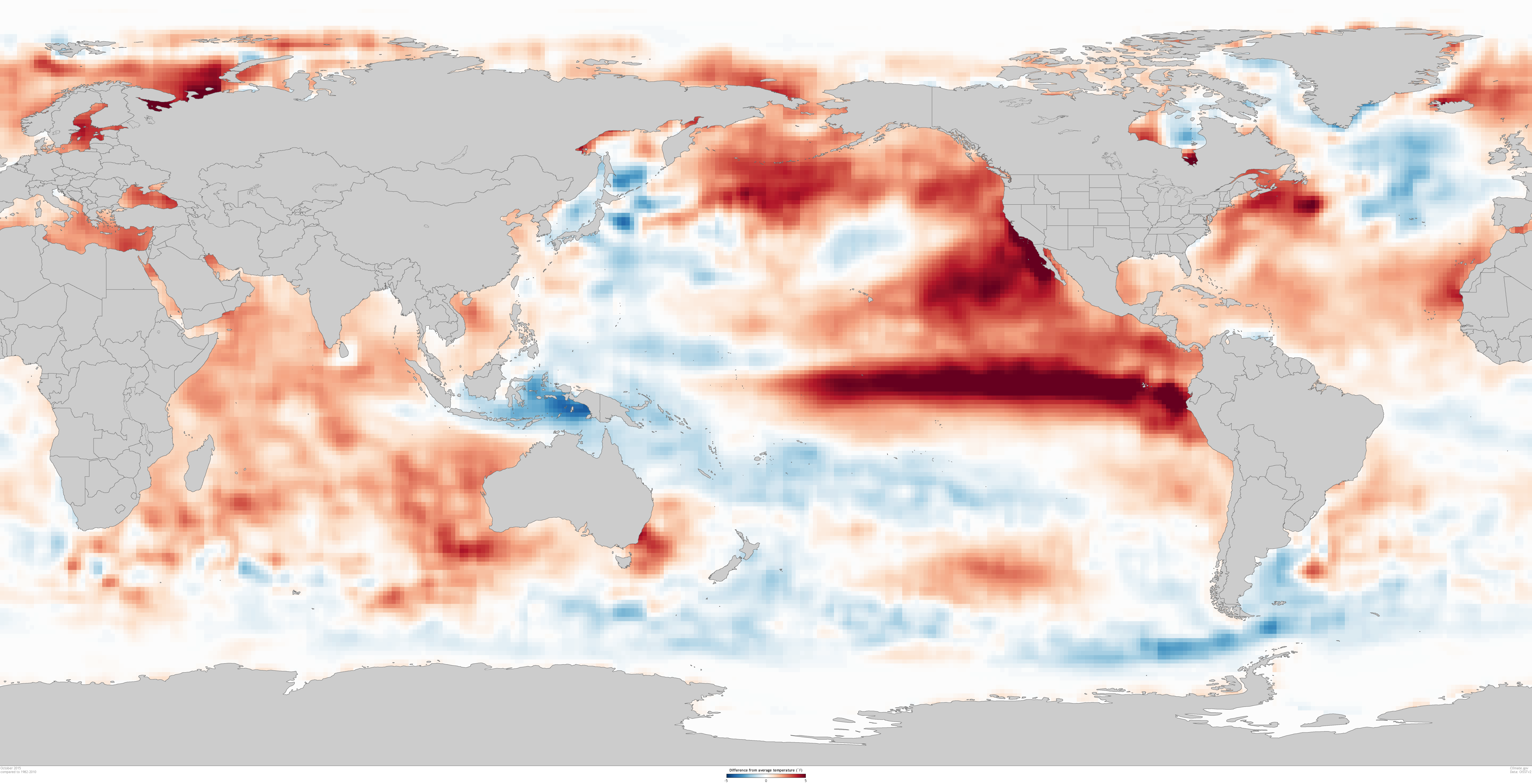
Comparison between two sea surface temperature datasets for the month of October 2015. On the left is the sea surface temperatures from the ERSSTv4 dataset. On the right is the monthly value of the averaged weekly OISSTv2 dataset. While similar in spatial pattern of sea surface temperatures, the datasets differ in resolution and data ingested. Graphic by climate.gov, data provided the Climate Prediction Center. large ERSSTv4 image | large OISSTv2 image
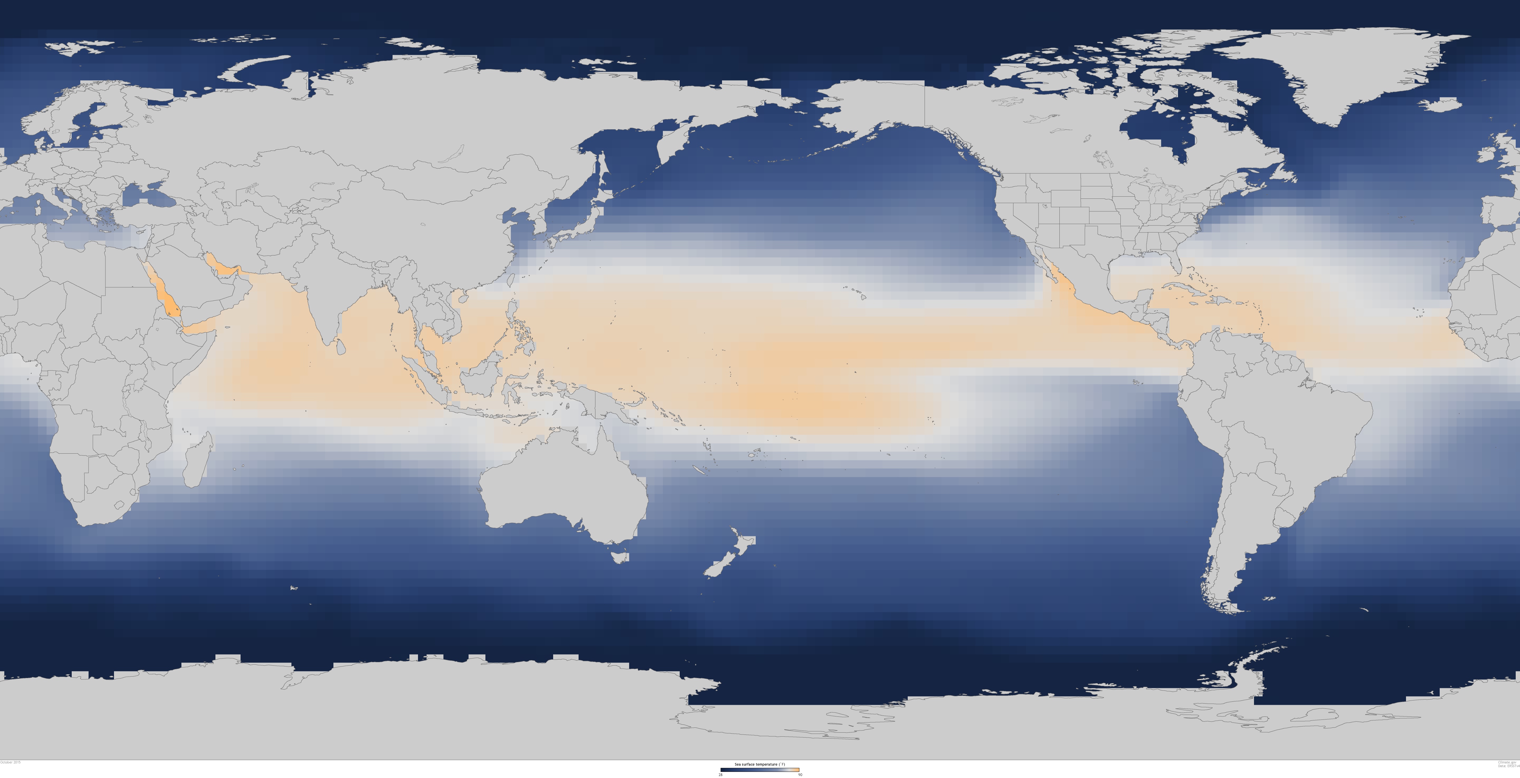
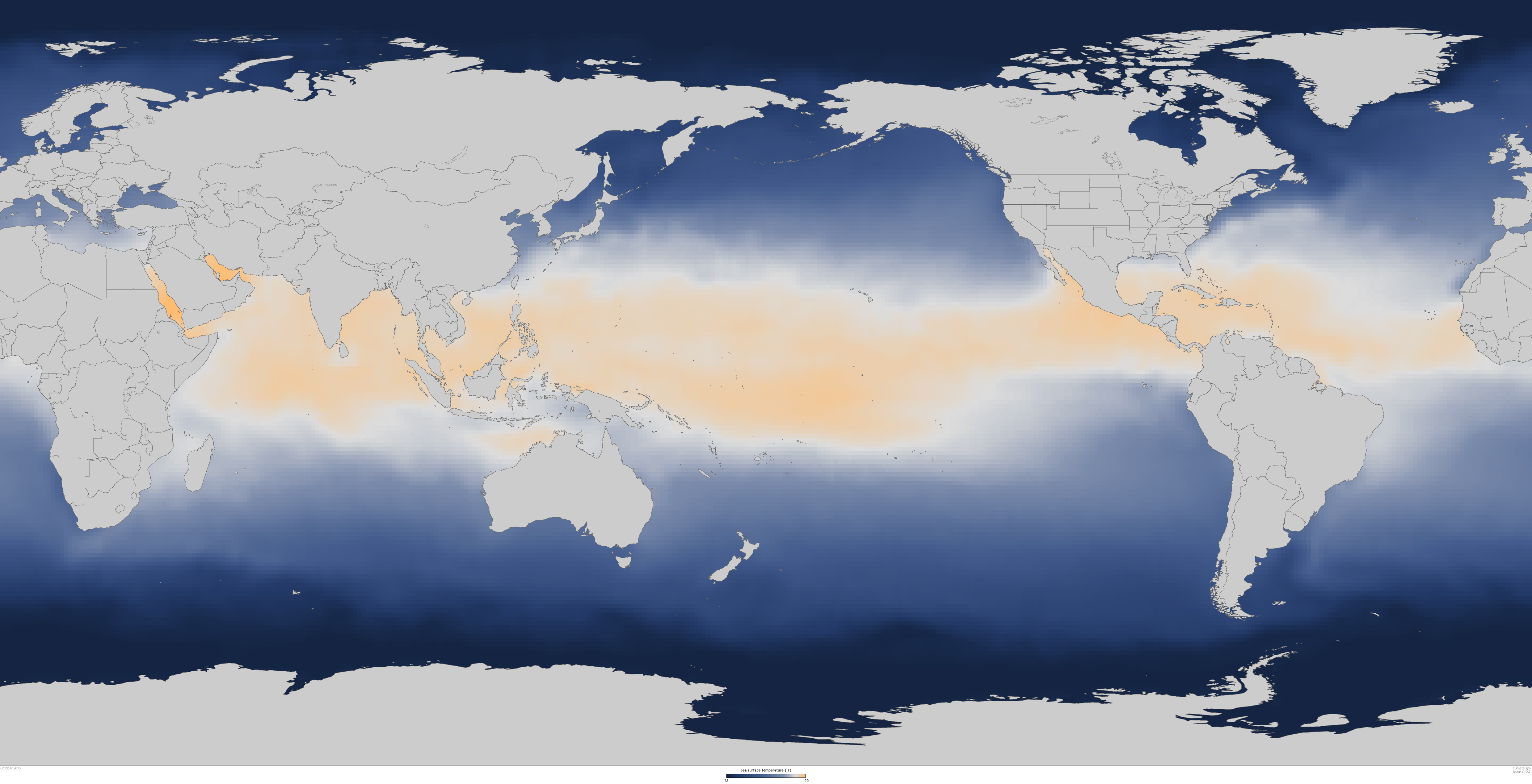
For historical comparisons, buckets, boats, and buoys
First, let’s look at the dataset that we use at CPC for all of our historical comparisons and forecast verification. The historical SST dataset is known as the ERSST v4, which is short for “Extended Reconstructed Sea Surface Temperature, Version 4.” (1). As its name implies, this dataset is reconstructed using ship and buoy information back to 1950 (2). The ship and buoy data is known as in situ, which is a fancy way of saying the data was measured at the location or “on site.”
The technology and methods for collecting water samples and taking temperature readings has changed over time. So scientists have painstakingly standardized the time series so that a 2.0°C anomaly in 1950, for example, is the same as a 2°C anomaly in 2015.
What kinds of things have to be corrected to standardize the dataset? Well, did you know that the way ships take water temperatures have changed? In the past, wooden, canvas or rubber buckets were used to gather ocean water. Nowadays, ships measure temperatures from water taken directly into the ship for the purposes of cooling the engines or the ships have sensors on their hulls. Water temperatures in buckets can be impacted by the surrounding environment including the type of material the bucket is made from, often biasing the measurements cool. Water that is taken into the engine room can be affected by how close it is to the ship’s engine or from how far at depth the water came from. Usually these measurements are biased on the warm side (Thompson et al. 2008).
Since this dataset relies on in situ observations, it is only updated once a month to allow for a larger number of observations to be reported over the month-long period. And there’s the problem: the models can’t wait a month.
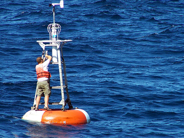
TAO buoy operations off the NOAA Ship Ka'imimoana. Electronics technician checking sensors on newly moored TAO buoy in the tropical Pacific Ocean. Photo by Lieutenant Commander Matthew Wingate, NOAA Corps.
Everything but the kitchen sink
ERSSTv4 goes back to 1854 (although due to a lack of observations in the Pacific Ocean, for El Niño purposes, the dataset reliably goes back to only 1950), and scientists have already put in a lot of time and effort to make this dataset consistent regardless of era (2). So why do we need another one? The easiest answer is that our seasonal climate models don’t run just once a month, but daily. Not surprisingly, they produce better forecasts when they are launched (we say “inititalized”) with a more detailed, more up-to-date view of what the oceans look like at that time.
For this situation, we want as much information as we can get it regardless of the historical consistency. So we rely on a dataset that combines in situ measurements with near-real-time satellite measurements. Satellites are not equipped with magical space thermometers that can measure the ocean temperature directly. Instead, instruments on the satellite detect energy radiating from earth to space. We use algorithms, physics equations and estimations to calculate what the sea surface temperature must have been to generate the amount of energy the satellite detected.
This dataset that we feed to the models is called the OISST, which is short for Optimal Interpolation SST. The SST part of the name should be self-explanatory, but Optimum Interpolation (OI) might need some clarification. OI is a statistical method for combining all the different forms of observations and fitting them onto a complete, gridded version of the world by interpolating (estimating) values at each of the grid points.
Multiple datasets can share the OISST moniker but actually refer to different datasets. OI is the method; the data ingested can be different. Just like how poaching is a cooking method but the taste of a poached egg versus a poached salmon will be very different. See footnote (3) for an explanation about why the daily OISST is actually a different dataset than the weekly OISST product.
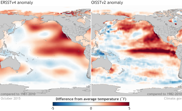
Comparison of sea surface temperature anomalies in two sea surface temperature datasets for the month of October 2015. On the left is the sea surface temperature anomalies from the ERSSTv4 dataset. On the right is the monthly value of the averaged weekly sea surface temperature anomalies in the OISSTv2 dataset. Graphic by climate.gov, data provided the Climate Prediction Center. large ERSSTv4 image | large OISSTv2 image
A satellite’s apples are a ship’s oranges
The benefit of OISST is that it is higher resolution (more geographic detail), and it is updated more than once a month. The problem comes when you attempt to use it to compare the strength of one event to another past event.
ERSST is carefully curated to keep everything on a level playing field, sacrificing satellite data and resolution to get it (4). OISST has less historical consistency with SST data before the satellite era (nominally starting in early 1980s). Plus, since satellites do not measure sea surface temperatures directly and the satellites in the 1980s were different than today, there are inherently biases added to the dataset within the satellite era. And while scientists do their best to remove them, the extent of the biases is a bit of an unknown. No correction can account for all of them. So, when we want to compare the OISST Niño3.4 anomaly to 1997 or any other past event, OISST would not be our best choice (5).
So the next time you want to compare the strength of this El Niño with past historical cases, use the ERSSTv4 dataset, compiled from buckets, boats, and buoys. That is what it was created for. But if you want to see the smaller-scale spatial and more frequent temporal changes of sea surface temperatures that occur within an event, OISST is more useful.
Footnotes
(1) ERSST stands for the Extended Reconstructed Sea Surface Temperature dataset and is updated and maintained by our colleagues at the National Centers for Environmental Information.
(2) The dataset is extended back in time to 1854. However, since there is a more severe lack of ship and buoy data the farther back you go, the ocean temperatures become less reliable to use as a source of comparison. The Pacific Ocean is a huge place where for much of history not much was being measured (see Figure 3 in this paper for a great illustration of this). 1950 has been determined to be a reasonable cutoff point where measurements are consistent both in terms of space and time across the Pacific for the determination of sea surface temperature anomalies in the Niño3.4 region.
(3) At CPC there is a daily OISST dataset that is used in our models. However, this is a more recent product. Before the daily product existed, there was (and still is) a weekly OISST dataset. This weekly product is different entirely and is not simply the seven-day average of the daily OISST for a variety of reasons (see references below). Since both of these products are satellite-based -- they do not measure sea surface temperatures directly -- there are adjustments done before we get the final SSTs (these adjustments change from month to month). Different methods and statistical techniques in the daily and weekly product lead to different numbers in the two similarly named datasets. For instance, ship and buoy SSTs are measured differently and at slightly different water depths, thus there is a statistical difference of ship-buoy SSTs of about 0.12ᵒC. The weekly OISST was developed when ships were the main source of in situ observations, and there is no ship-buoy SST adjustment in it. On the other hand, the latter daily OISST was developed when more buoy data became available, and there is a ship-buoy SST adjustment in it, as in the latest version of ERSST.
(4) ERSST, for instance has a grid point every 2° while the higher resolution daily OISST has a grid point every 0.25° and weekly OISST is 1°.
(5) If you want to compare Niño3.4 values amongst the different datasets for a single month, treat them like you are a contestant on Price is Right and you are gathering estimates from the crowd on a new dishwasher. No estimate is likely “right” but you can get a ballpark figure or a range on the price. And, of course, some audience feedback, like from your best friend the dishwasher salesmen, could be weighed more so than others. After all, buoys, ships and satellite SST observations will be slightly different from each other because they incompletely measure the vastness of the Pacific Ocean while biases that exist within the dataset will skew the final Niño3.4 numbers. This concept of uncertainty is why in reality, the Niño3.4 numbers from each dataset should not be seen as just a number but as the center point of a range. So, if you’re curious about the actual number for a certain moment in time, it is best to look at all of these datasets as displaying a range of possibilities and not as one “right” answer” and four wrong ones. When taking into account each dataset’s uncertainty what at first appears to be a large difference between SST datasets might not be that large after all. Figuring out, though, just how much uncertainty exists in these datasets, especially in the satellite-based OISST datasets, is an active area of research.
A special thanks to Boyin Huang, Viva F. Banzon, Huai-Min Zhang and Deke Arndt at the National Center for Environmental Information (NCEI) for their help in reviewing this piece and providing additional information needed to make this post complete.
References
Thompson, David W.J., J.J Kennedy, J.M. Wallace, P.D. Jones, 2008: A large discontinuity in the mid-twentieth century in observed global-mean surface temperature. Nature, 453, 646-649
ERSSTv4
Boyin Huang, Viva F. Banzon, Eric Freeman, Jay Lawrimore, Wei Liu, Thomas C. Peterson, Thomas M. Smith, Peter W. Thorne, Scott D. Woodruff, and Huai-Min Zhang, 2015: Extended Reconstructed Sea Surface Temperature Version 4 (ERSST.v4). Part I: Upgrades and Intercomparisons. J. Climate, 28, 911–930.
Wei Liu, Boyin Huang, Peter W. Thorne, Viva F. Banzon, Huai-Min Zhang, Eric Freeman, Jay Lawrimore, Thomas C. Peterson, Thomas M. Smith, and Scott D. Woodruff, 2015: Extended Reconstructed Sea Surface Temperature Version 4 (ERSST.v4): Part II. Parametric and Structural Uncertainty Estimations. J. Climate, 28, 931–951.
Daily OISST
Richard W. Reynolds, Thomas M. Smith, Chunying Liu, Dudley B. Chelton, Kenneth S. Casey, and Michael G. Schlax, 2007: Daily High-Resolution-Blended Analyses for Sea Surface Temperature. J. Climate, 20, 5473–5496.
Viva F. Banzon, Richard W. Reynolds, Diane Stokes, and Yan Xue, 2014: A 1/4°-Spatial-Resolution Daily Sea Surface Temperature Climatology Based on a Blended Satellite and in situ Analysis. J. Climate, 27, 8221–8228.
Weekly OISST
Reynolds, R. W., and T. M. Smith, 1994: Improved global sea surface temperature analyses using optimum interpolation. J. Climate, 7, 929–948
Reynolds, R. W., N. A. Rayner, T. M. Smith, D. C. Stokes, and W. Wang, 2002: An improved in situ and satellite SST analysis for climate. J. Climate, 15, 1609–1625.
ERSST and OISST Comparisons
Huang, B., W. Wang, C. Liu, V. F. Banzon, J. Lawrimore, and H.-M. Zhang, 2014: Bias adjustment of AVHRR SST and its impacts on two SST analyses. J. Atmos. Oceanic Technol., 32, 372-387, doi:10.1175/JTECH-D-14-00121.1
Boyin Huang, Michelle L’Heureux, Jay Lawrimore, Chunying Liu, Huai-Min Zhang, Viva Banzon, Zeng-Zhen Hu, and Arun Kumar, 2013: Why Did Large Differences Arise in the Sea Surface Temperature Datasets across the Tropical Pacific during 2012? J. Atmos. Oceanic Technol., 30, 2944–2953. doi: http://dx.doi.org/10.1175/JTECH-D-13-00034.1
Comments
Precision and accuracy can be compromised?
An enlightening notes
The Article That I've Been Looking For
RE: The Article That I've Been Looking For
Glad it was useful to you! Also, we don't weight weekly values of SST much because ENSO is best seen in seasonally (3 month) averaged data: https://www.climate.gov/news-features/blogs/enso/keep-calm-and-stop-obsessing-over-weekly-changes-enso
Add new comment