When it comes to probabilities, don’t trust your intuition. Use a decision support system instead!

This is a guest post by Brian Zimmerman, a climate scientist at Salient Predictions. Salient is a startup that utilizes advances in machine learning and artificial intelligence to develop and provide accurate, reliable forecasts on the subseasonal-to-seasonal timescales. Additionally, Brian serves as a decision support specialist, helping clients to navigate uncertainty in the most effective manner possible.

The nature of uncertainty

There are not too many things more frustrating in this world than unmet expectations. Your favorite basketball team has an estimated 79% chance of beating the upcoming opposition; yet, they lose, and you’re out $10 to your work betting pool. There was only a 15% chance of rain in the forecast one day before your friend's wedding, and it starts raining precisely 10 minutes before the outdoor ceremony is supposed to start. Or perhaps you’re in the ENSO betting market.

Regular readers of the blog recognize that climate predictions are uncertain, including for the El Niño-Southern Oscillation (ENSO), which are expressed as probabilities (70% chance of El Niño coming) instead of forecasting a single black-and-white outcome (El Niño is coming). To make decisions in the face of uncertainty, we sometimes consciously, often automatically, use our best guess at how likely the various outcomes are and what our tolerance for risk in the given situation is. For all but a few of us (nerd alert!), this is done in a qualitative, intuitive fashion. 

The trouble is, humans aren’t very good at it. Most of us find it difficult to intuitively understand probabilities except 0, 50, and 100%. In order to make sense of an uncertain world, we often craft narratives that enable us to make decisions and move forward. Unfortunately, these narratives tend to be compromised by two traits: our penchant for overconfidence and our aversion to risk (see footnote #1). This generally leads us to sorely misestimate the likelihood of almost all events facing us as we move through our lives. An even more frustrating truth to face is that even if we correctly act on probabilistic information (know the true odds of a given event and make the best decision possible) the outcome may be opposite of what we favored.

So, what to do? This blog post aims to offer some tips and tricks that are likely to lead to greater fulfillment of all your most accurately estimated dreams! Let’s learn from a simple example. I’ll use a sports betting analogy to highlight the benefits of using calibrated probabilistic forecast models (like the CPC ENSO forecast!) for real-world decisions.

Betting on the Bulls: building a decision support system

Say you're a Bulls fan, and there’s a betting pool at work. Given no information about them or their competition, you would assume that the odds that they win any given game is 50-50. In reality, not all teams are equally matched, so the true chances the Bulls will win a given game will vary. To maximize your odds of large profits over the season, you need a system for guiding how much to bet based on a range of probabilities. Good probabilistic decision making requires two key items (see footnote #2 for additional commentary): 

1) A clearly defined event with a yes-no outcome:

The Bulls will win their game tomorrow night.

2) A set of actions you’ll take at specific thresholds:

This table shows what you will gamble based on what you think the probability is of the Bulls winning against whatever team they are playing. The maximum you can put into the pool is $50. 

Your decision support system (DSS) for determining how much to bet based on your estimate of the percent chances of the Bulls beating their opponent. 

If the odds are less than 50%, you don’t risk your money. The higher the odds above 50%, the more you bet. (Note: this table above is your decision support system or DSS.)

Now that we have our DSS, we can mock up how this system would work out in 3 situations: 

1. a scenario where you know absolutely nothing about basketball, and don’t try to learn. You just bet randomly based on what you had for lunch that day. This is akin to using the Farmer’s Almanac to forecast ENSO. 
2. a scenario where you are an experienced basketball enthusiast with a discerning eye. Your estimation of the true probabilities of the Bulls winning against any team they play is perfect. This would be equivalent to climate scientists having a model that perfectly predicts the chances of El Niño in a given season: for instance, when the model predicts there is a 70% chance of El Niño coming, El Niño actually happens 70% of the time.
3. a scenario where you’re enthusiastic and like sports, and your estimation of the true probabilities of the Bulls winning against any team they play is good, but not perfect. This would be equivalent to climate scientists having a model that does not perfectly predict the chances of El Niño, but is pretty good! For instance, when the model predicts an 80% chance of El Niño coming, El Niño actually happens 60% of the time. 

How would you wind up in each of these situations? I worked up some code (see footnote #3) so we can explore the outcomes!

Outcomes!

Each experiment simulates 1,000 seasons of 82 games each. The tables below show excerpts from one season of the second (perfect estimates of the chances of winning) and third experiments (estimates of the odds of a Bull’s victory are good, but not perfect.)

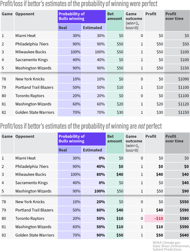
(top) A simulated season in Experiment 2, where if you predict the Bulls have a 90 percent chance of winning a game against the 76ers, they do, in fact, win against them 90% of the time (line 2).  (bottom) A season from Experiment 3, where your estimates of the chances are good, but not perfect. You estimate the Bulls have a 60% percent chance of beating the Wizards over time, but they only beat them 50 % of the time (Line 81).  NOAA Climate.gov graphic, based on data from Brian Zimmerman. 

The bar charts below shows the results of the experiments. The top row is experiment 1 (random betting), the middle is Experiment 2 (you predict the Bull’s chance of winning perfectly), and the bottom is Experiment 3 (good, but not perfect.)

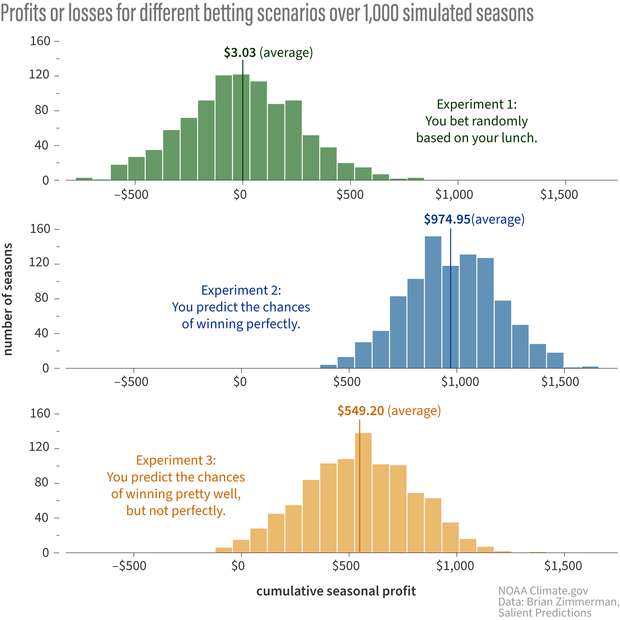
Each bar chart shows the cumulative profit or loss from betting after 1,000 simulated basketball seasons. The amount of profit or loss is shown across the bottom of the chart, and the height of the bar indicates how many seasons had that total. When you bet randomly (top), you lose as often as you win, and your average profit is close to zero.  When you bet following a decision support system that risks more when you think the Bulls' odds of winning are higher, you make more than $500 on average even if you can't predict their odds of winning perfectly (bottom). NOAA Climate.gov image, based on data from Brian Zimmerman. 

The first thing to notice is that by simply utilizing a tailored decision support system (DSS), you can come out ahead over time even if all you know is the probability of your team winning a game. The figure above makes this obvious; randomly betting performs much worse overall! Yes, sometimes the Bulls lose when the chance of winning is high, but if you stick to the program (your DSS), you will end up ahead at the end of the season (in this simulation, see footnote #4).

Now, you might be saying to yourself, “Okay, sure, you can come out ahead if you know the probabilities perfectly, but no one actually knows the true odds of their team winning any game.” Not to fear! The bottom row of the graphic shows that, over the long haul, the consistent implementation of decisions derived from your DSS is almost always lucrative even when your forecasts are not perfectly reliable! It’s the DSS that is critical here.

Comparing the three experiments, we see something we’d expect—that using a decision support system based on perfect knowledge of the probabilities is the MOST lucrative. But we can also see something that is perhaps not intuitive: the figure below shows that over shorter periods of time, our imperfect estimates (or even random bets!) will sometimes put us further ahead than using perfect estimates of the odds.

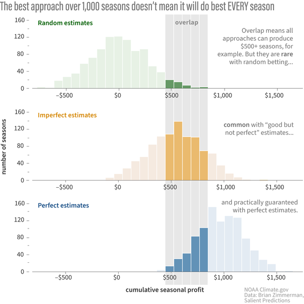
Out of a thousand seasons, there will be some where random betting (top) or imperfect estimates of the chances of winning (middle) will make as much money as betting with perfect knowledge of the probabilities (bottom). Inevitable negative outcomes can be one of the hardest things for people to accept about forecasts that use probabilities. NOAA Climate.gov image, based on data provided by Brian Zimmerman. 

That is because there is still some randomness in the actual outcomes of the game (see footnote #3 on “noise”). A 60% chance of victory means that you will lose your bets on occasion (60% does not equal 100%). It's inevitable that there will be a single game, or even 5- or 10-game stretches (possibly even an entire season!), where you actually end up with higher profits using a DSS with imperfectly estimated probabilities or even just random bets.

This is shown in a different way in the line graph below. I cherry–picked a season that shows both Experiment 1(random guesses) and Experiment 3 (good, but not perfect estimates of the true probability) performing worse than Experiment 2 (perfect prediction of the probability)—but only for the 1st half of the season! In the end, if you follow your DSS, you end up much better off than randomly betting, even with imperfect estimation of the probabilities.

Game by game cumulative profits for season 796 from each of the three experiments. In this season of the experiments, the bettor scenario using a decision support system with true probabilities (blue) did worse than the other two strategies until the very end of the 82-game season! NOAA Climate.gov image, adapted from original by Brain Zimmerman.

Bringing it all together

This simple example shows how we can benefit from uncertain, probabilistic estimates of the chances a team will win a game. As frustrating as it may be, a single bad game or even one bad season doesn't mean our strategy is flawed. Making decisions based on weather, climate, and ENSO forecasts is similar! In fact, any probabilistic forecast is similar.

In ENSO forecasting, a premium is put on using so-called “calibrated” forecast models, which are constructed using long hindcasts to create more reliable outlooks. In calibrating the model output, the goal is to make the forecast estimates closer to the true probabilities - which pushes us closer to the case outlined by Experiment #2. This allows for the highest chance of the best outcomes over the long haul, but also by no means guarantees them.

Having a solid DSS means we also have considered our tolerance for risk and how to act upon the estimated forecast probabilities. This should help us avoid disappointment and stay true to the course when we don’t get an outcome we hoped for. In an inherently uncertain world, it’s the best we can do.

Lead editors: Rebecca Lindsey and Michelle L'Heureux. 

Footnotes

1. Some additional reading: 
   Kahneman, Daniel. (2011). Thinking, Fast and Slow. London: Penguin Books. 
   Here's a related Guardian article/interview with Kahneman where he states that if he could wave a magic wand and eliminate one thing, it would be "overconfidence." 
   Kahneman and Tversky (1979). Prospect Theory: An Analysis of Decision under Risk. Econometrica, 47 (2), 263-292. 
2. Event Definition:
   An event can literally be anything! However, whatever you choose, it’s critical to be specific. It could be something like “the Bulls will win tomorrow's game against the 76ers”, or “El Niño will develop between now and March 1st” - essentially, anything that can have a definitive outcome of either “yes it did happen” or “no it didn’t happen”. 

   Thresholds of Actionability: Here is where it gets tricky. The goal for defining “thresholds of actionability” is to determine a set of actions you would take given the various probabilities of the defined event occurring. This can be complicated because it starts to incorporate all kinds of other concepts - and is highly prone to the influence of Narrative. It’s also highly personal because different people or organizations have different risk tolerances! Ideally, these thresholds of actionability would be defined and analyzed over some historical period in order to optimize the thresholds, but let's leave that alone for now and just make up some that seem reasonable. We can go back to our sports example for some simple fun.

3. I created a Betting Simulator to generate these experiments. You can run it yourself because I put the python code here: https://github.com/bgzimmerman/enso_blog. The results in this blog are generated from the output of 1000 synthetic seasons of betting in the pool. There are 82 games in a season - the true probability of the Bulls winning is created using a stochastic generator - your estimated probability (on which you cast a bet) is generated conditioned on the true probability. For simplicity, the profit on a win is equivalent to the bet placed. We explore two scenarios - one in which you are perfectly prescient (i.e. your estimated probability equals the true probability) and another in which we incorporate estimation error (a tunable parameter - it adds noise to the true probability to create your estimated probability). The addition of noise here is meant to emulate both the impact of having an imperfect model and how human Narrative can lead you astray from the true probabilities (i.e. “Oh they lost the last two games so they’re due for a win this time!”). 

   Additional Notes: In this simple example, we’re not getting into issues of who pays out the bet, what are the house odds, etc. In real betting, a gambler allocates bets based on having an edge. Finally, reliable probabilities will give you a higher payout but only if the scoring is “proper” (see Brocker and Smith, 2007 and Gneiting et al., 2007).

4.  Astute readers may note that in this simulation with the true probabilities there is not a single season of 82 games in Experiment 2 where you lose money. Even in Experiment 3 (estimated probabilities) you don’t often lose money over a full season. However, do not jump to the conclusion that as long as you know a little bit about the sport, betting for a full season will return some money! This outcome is a result of the assumptions in the Betting Simulator. The simulator could be easily adjusted so there are more opportunities to lose money. Download it and experiment yourself if interested!