Will La Niña follow El Niño? What the past tells us
As the strong El Niño begins weakening later this winter and spring 2016, some clever folks may wonder whether La Niña conditions might develop in the second half of the year. The figure below shows the variations of the 3-month average sea surface temperature departures from average (the anomaly) in the Niño3.4 region, using the ERSSTv4 data (footnote 1).

Plot of running 3-month average sea surface temperature (SST) in the Nino3.4 region (called the ONI), using the ERSSTv4 SST data. See footnote (1) and Tom’s blog for more detail about the ERSSTv4 data.
You can see that sometimes La Niña does occur the year after a significant El Niño, like after the El Niño events of 1997-98, 1972-73 and 2009-10. But it doesn’t always happen, such as after the events of 1991-92 and 2002-03.
Can we estimate how likely a switchover is from an El Niño to a La Niña for the following year? And does it depend on how strong the El Niño is? I’ll try to answer this question using relationships based on past data from 1950 to present.
Look to the past
I start by rating each year’s ENSO state – that is, if it’s El Niño, La Niña, or neither, and how strong. Then I classify each year’s average anomalies of at least 0.5° but less than 1.0° Celsius as being a weak El Niño, at least 1.0° but less than 1.5° a moderate El Niño, and 1.5° or greater a strong El Niño. (See footnote 2 for how the rating is made.)
Given that El Niño only occurs every few years, we have a fairly short historical record from which to draw inferences, which is why the analysis I present here needs to be put in context alongside other forecast tools, including computer models and the official ENSO forecasts.
The tables below show what ENSO conditions have followed each of the seven moderate and the three strong El Niño events since 1950. In six out of the ten cases, the sea surface temperature was -0.5° C or cooler than average, satisfying the definition used here for La Niña (footnote 3). For the three strongest events, all resulted in La Niña based on this method of classification. But how convincing is this? Would we want to put money on a La Niña prediction?
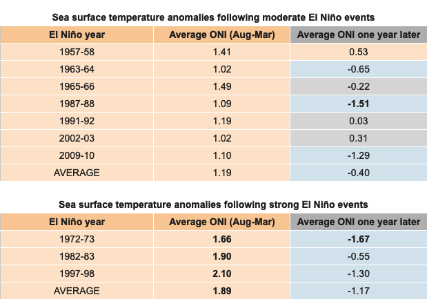
ENSO conditions observed the year following a moderate (top table) or strong (bottom table) El Niño during 1950-2015. The numbers in the table are the average of the ONI SST data (degrees C) for the six 3-month seasons of ASO, SON, OND, NDJ, DJF and JFM. Orange shading indicates El Niño years, blue indicates La Niña years, and bold values indicate an SST anomaly strength of at least 1.50 degrees C (our strong event category).
Numbers!
When looking at the results for weak, moderate, and strong El Niño separately, I find an average sea surface temperature anomaly of -0.15 °C the year after the 11 weak El Niños, -0.40 °C after the 7 moderate El Niños, and -1.17 °C for the 3 strong El Niños.
These averages do suggest that stronger El Niño events have a higher likelihood for a La Niña the following year. But not so fast! It’s always possible that the pattern I found is simply a coincidence. To test the likelihood that these mean differences reflect true underlying differences, I threw all 21 cases together (11, 7, and 3 cases for weak, moderate and strong El Niño, respectively), and computed the correlation (footnote 4) between the strength of El Niño during the first year and the sea surface temperature state the following year.
The resulting correlation is -0.31, which translates to a very weak tendency for the sea surface temperature the following year to be colder when the El Niño the first year is stronger (footnote 5). We can use this relationship to make a rough statistical prediction of the ENSO state next year (see footnote 6).
It’s a safe bet that the sea surface temperature departure this year will be greater than 1.5°C even though we don’t yet have 3-month data through January-March 2016. According to this analysis, the best guess for the 2016-17 ENSO state would be within the weak La Niña category (footnote 6 again; see the figure below, and the caption).
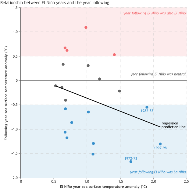
Scatterplot showing the relationship between the ENSO state (using the 6-running-season ONI definition) for years having an El Niño (x-axis), and the ENSO state the following year. Each dot represents one pair of “year 1 vs. year 2” ENSO states for El Niños observed since 1950. The downward sloping line is a simple linear regression fit to the data points, defined so that the square of the errors (the vertical distance from each point to the line) is mathematically minimized. A forecast for the ENSO state for the year following an El Niño can be made using the line, by setting the x-axis value to the ENSO state value for the El Niño year, and finding the y-axis value of the line for that x-axis value. For example, if the ENSO state for the first (El Niño) year is 1.8, the estimate for the ENSO state for the next year would be about -0.8. The high standard error, and thus high uncertainty (see footnotes 6 and 7), is caused by the large errors of the points with respect to the line—i.e., many of the points are far above or below the line. That high uncertainty is indicated by the weakness of the correlation coefficient (-0.31) for the points in the scatterplot.
But the fly in the ointment in this “forecast” is its large uncertainty, illustrated by how a lot of the points are not near the line. This uncertainty can be described mathematically by using the standard error of estimate (footnote 7), which tells us the size of the error tolerance, and says that the probability of getting La Niña for 2016-17 is 66%, leaving a 34% chance for falling short of the La Niña threshold.
The large uncertainty of this method is why forecasters don’t just look at the past to predict the future, but also take into account other prediction tools, including state-of-the-art computer models that consider a more comprehensive set of features relevant to ENSO prediction.
Physics!
Aside from doing this number crunching on the historical observations, there are accepted physical reasons for expecting a tendency toward La Niña the year after a significant El Niño. One of these is the delayed oscillator theory, introduced in 1988 by Suarez and Schopf.
The theory says that the low-level westerly wind anomalies, a hallmark of El Niño, not only trigger eastward-moving oceanic Kelvin waves at the equator (see Michelle’s blog), but also westward-moving waves just north and south of the equator (called Rossby waves). While Kelvin waves are pushing warm water east, these Rossby waves move cooler subsurface water toward the west. They then bounce off the western side of the tropical Pacific (around Indonesia) and have a return trip, traveling eastward near the equator.
On their eastward trip, these waves also promote cooler water, and can neutralize or reverse El Niño around 6 months after the westerly wind bursts. This cool pulse interrupts the positive feedback mechanism responsible for the growth of an El Niño, ending El Niño and promoting La Niña development.
Since stronger El Niño events often involve stronger westerly wind anomalies, these events tend to trigger stronger Rossby waves and stronger tendencies for El Niño to decay and possibly reverse after peaking at the end of a calendar year.
Based on the statistics derived from the historical data and on the more physical basis as described by delayed oscillator theory, the CPC/IRI team is expecting some cooling coming up in 2016-17. So, stay tuned to upcoming ENSO outlooks (footnote 8)!
Footnotes
(1) ERSSTv4 stands for Extended Reconstructed Sea Surface Temperature, version 4. As discussed in more detail in Tom’s recent blog, its 3-month average SST data, called the ONI (for Oceanic Nino Index) is developed with the purpose of preserving homogeneity throughout the last 60 or more years, despite changes in SST measurement methods and the relatively poorer SST data coverage before satellites came along in the early 1980s. This homogeneity is a main reason that the ERSSTv4 SST data is officially used by NOAA/Climate Prediction Center for ENSO diagnosis and for comparisons between any years from 1950 to present. An alternative SST dataset is called OISST (Optimum Interpolation SST), which combines satellite and direct gauge measurements of SST. While OISST is more modern and considered more state-of-the-art by some, it has problems such as variable satellite measurement biases and other issues that can create inhomogeneities over time and space. The OISST is used to initialize models and to detect changes in SST on shorter time scales (e.g. week-to-week) and spatial scales.
(2) To ensure that El Niño events with differing timings are captured, the six three-month periods that have the strongest average anomaly when the anomaly is positive, are averaged. These turn out to start with August-October and end with January-March.
(3) Note that the ENSO definitions used here are only for the purpose of this examination. NOAA CPC defines an El Niño episode as an event in which the SST anomaly of 0.5 °C or greater in the Nino3.4 region persists for at least 5 consecutive 3-month overlapping seasons, and there are no official ENSO strength definitions. The informal strength definitions that NOAA uses have the same cutoffs as those used here, but are for just the peak single 3-month period, not for the average of six periods. By averaging together ASO, SON, OND, NDJ, DJF and JFM, we may define some years as ENSO events that are not formally classified. The cool period of 1983-84, for example, passes our test for a weak La Niña (at -0.55 C) but did not formally qualify because its period of maintaining at least a -0.5 anomaly was too brief.
(4) A correlation coefficient tells us how closely related two variables are. Here, the variables are (1) the ENSO state the first year and (2) the ENSO state the following year. A correlation of 1.0 implies a perfect relationship between the two variables, so that knowing the ENSO state the first year would give us a perfectly accurate prediction of the ENSO state the next year, and the two variables vary in the same direction as one another (warmer SST in first year means warmer SST the year afterwards). A correlation of -1.0 also implies perfect predictability, except that the two variables move in opposite direction to one another; i.e., the warmer the SST during the first year, the colder it will be the second year. A correlation of 0.0 means that the two variables are totally unrelated to one another. Usually, correlations are somewhere in between these numbers, and imply some relationship between the two variables, but with some uncertainty as well. Correlations weaker than 0.5 (or -0.5) suggest just a weak relationship.
(5) A test of statistical significance (to be explained momentarily) for this correlation of -0.31 indicates that the probability that the true correlation (i.e., the correlation we would get if we had an infinitely large sample of cases) is negative is 92%, and that it is not negative is 8%. The 92% probability suggests the true correlation is negative, but with moderate uncertainty. We normally want to see at least a 95% probability to be confident in our correlation. A statistical significance test for a correlation tells us the probability that it could have occurred by chance, and that the true correlation is zero (or even in the opposite direction from the sample result). Statistical significance becomes more difficult to obtain the smaller the number of cases in the sample, and the weaker the strength of the correlation (whether positive or negative). The correlation strength is diminished when the case-to-case variability is large compared with the overall relationship between the two variables. In our case, the significance is on the weak side because of the weak correlation (-0.31) combined with the somewhat small sample size of 21 cases.
(6) This method of analysis is called simple linear regression. This simple linear regression forecast is derived from the relationship between the ENSO state (using our 6-running-season average ONI definition) using years having at least a weak El Niño, and the ENSO state the following year. The figure shows the line that best fits the data points, where the square of the errors (the vertical distance from each point to the line) is mathematically minimized. We can then use the regression line to find what the best guess for next year’s ENSO state will be (the y-axis value on the line, where the x-value is greater than 1.5°C; we will know it exactly after March 2016). The standard error of estimate (see footnote 7), based on the correlation coefficient of only -0.31, is high, indicating large uncertainty of the forecast. The high uncertainty is consistent with the large errors of the points with respect to the line (many of the points are far above or below the line rather than close to it).
(7) The standard error of estimate tells us the amount of uncertainty in the forecast. The weaker the correlation coefficient between the first variable (often called the predictor) and the second one (called the predictand), the larger the standard error. So, if the correlation is -1 or +1, the standard error is 0 (no uncertainty; the numerical forecast would have perfect accuracy), and if the correlation is 0, the standard error is the largest possible, and equals the uncertainty of the predictand if we had no predictive information at all; that is, it is just the historical variability of the predictand, per se.
(8) Note that this blog does not constitute an official NOAA ENSO forecast. That official NOAA forecast is discussed here, with forecast probabilities for La Niña, neutral and El Niño, at least out to August-October 2016, given here. The NOAA forecast does hint toward La Niña, but we will need to wait another couple of months to see what it says about seasons closer to the usual peak in late autumn 2016.
References
Suarez, M. J., and P. S. Schopf, 1988: A delayed action oscillator for ENSO. J. Atmos. Sci., 45, 3283-3287.
Comments
Question on Blog post
RE: Question on Blog post
Seasonal values are used because the weekly data is not a homogenized data set. Therefore differences among various events might result from differences in the data sets and not be physically based.
RE: RE: Question on Blog post
I will also add that even if the weekly was homogenized, we still wouldn't use it to define El Nino. That's because El Nino is a seasonal (3 month average) climate phenomenon that is best identified on those timescales. More on this topic is here: https://www.climate.gov/news-features/blogs/enso/keep-calm-and-stop-obsessing-over-weekly-changes-enso
Ninio - Ninia
RE: Ninio - Ninia
Yes-- that's right. If the statistics based on the past do not continue to the future, then there will be an unknown error associated with that. With that said, at this point it is not clear that ENSO has changed under global warming (can read the latest IPCC AR5 sections for more), so statistical prediction methods of ENSO are still pretty useful.
Updates
RE: Updates
There will not be updates on this particular forecast based on regression. But each month the Climate Prediction Center issues another forecast for the coming ENSO conditions out to about 10 months in advance, and at the time I'm writing this (middle February), those ENSO outlooks go out to Oct-Nov-Dec 2016, which should be plenty of time to capture the possible La Nina development. The link to their latest forecasts is given in the last footnote in this blog. Right now, they actually do show a 50% chance for La Nina development for Oct-Nov-Dec 2016, somewhat in agreement with the regression forecast given above.
As for studies of big storms like Mitch and other high impact events, there have been studies related them to the ENSO condition. I am not in a position right now to name more than one, but there are many, and you would need to probe into the scientific literature about ENSO and such big weather events. The one article I do know is the following: Authors: Lisa Goddard and Maxx Dilley: "El Nino: Catastrophe or Opportunity?" Journal of Climate, Volume 18 (March 2005), pages 651–665.
average high & low tempitures for 1880
RE: average high & low tempitures for 1880
Hi David, That's a question for NCEI user services. (NCEI is the part of NOAA that archives and distributes climate data).
https://www.ncdc.noaa.gov/contact
Add new comment